Tutorial: Repeated Measures
Source:vignettes/tutorial_repeated_measures.Rmd
tutorial_repeated_measures.RmdThis vignette documents how dabestr is able to generate
estimation plots for experiments with repeated-measures designs.
dabestr allows for the calculation and plotting of effect
sizes for:
- Comparing each group to a shared control (control vs. group i;
baseline) - Comparing each measurement to the one directly preceding it (group i
vs group i+1;
sequential)
This is an improved version of paired data plotting in previous versions, which only supported computations involving one test group and one control group.
To use these features, you can simply declare the argument
paired = "sequential" or paired = "baseline"
correspondingly while running load(). You must also pass a
column in the dataset that indicates the identity of each observation,
using the id_col keyword.
Create dataset for demo
set.seed(12345) # Fix the seed so the results are replicable.
# pop_size = 10000 # Size of each population.
N = 20 # The number of samples taken from each population

# Create samples
c1 <- rnorm(N, mean = 3, sd = 0.4)
c2 <- rnorm(N, mean = 3.5, sd = 0.75)
c3 <- rnorm(N, mean = 3.25, sd = 0.4)

t1 <- rnorm(N, mean = 3.5, sd = 0.5)
t2 <- rnorm(N, mean = 2.5, sd = 0.6)
t3 <- rnorm(N, mean = 3, sd = 0.75)
t4 <- rnorm(N, mean = 3.5, sd = 0.75)
t5 <- rnorm(N, mean = 3.25, sd = 0.4)
t6 <- rnorm(N, mean = 3.25, sd = 0.4)

# Add a `gender` column for coloring the data.
gender <- c(rep('Male', N/2), rep('Female', N/2))

# Add an `id` column for paired data plotting.
id <- 1:N

# Combine samples and gender into a DataFrame.
df <- tibble::tibble(
  `Control 1` = c1, `Control 2` = c2, `Control 3` = c3,
  `Test 1` = t1, `Test 2` = t2, `Test 3` = t3, `Test 4` = t4, `Test 5` = t5, `Test 6` = t6,
  Gender = gender, ID = id)

df <- df %>%
  tidyr::gather(key = Group, value = Measurement, -ID, -Gender)
Loading Data
two_groups_paired_sequential <- load(df, x = Group, y = Measurement,
                                     idx = c("Control 1", "Test 1"),
                                     paired = "sequential", id_col = ID)

print(two_groups_paired_sequential)
#> DABESTR v0.9.9.9
#> ================
#>
#> Good morning!
#> The current time is 04:27 AM on Tuesday August 22, 2023.
#>
#> Paired effect size(s) for the sequential design of repeated-measures experiment
#> with 95% confidence intervals will be computed for:
#> 1. Test 1 minus Control 1
#>
#> 5000 resamples will be used to generate the effect size bootstraps.
two_groups_paired_baseline <- load(df, x = Group, y = Measurement,
                                   idx = c("Control 1", "Test 1"),
                                   paired = "baseline", id_col = ID)

print(two_groups_paired_baseline)
#> DABESTR v0.9.9.9
#> ================
#>
#> Good morning!
#> The current time is 04:27 AM on Tuesday August 22, 2023.
#>
#> Paired effect size(s) for repeated measures against baseline
#> with 95% confidence intervals will be computed for:
#> 1. Test 1 minus Control 1
#>
#> 5000 resamples will be used to generate the effect size bootstraps.
When only 2 paired data groups are involved, assigning either
“baseline” or “sequential” to paired will give you the same
numerical results.
two_groups_paired_sequential.mean_diff <- mean_diff(two_groups_paired_sequential)
two_groups_paired_baseline.mean_diff <- mean_diff(two_groups_paired_baseline)
print(two_groups_paired_sequential.mean_diff)
#> DABESTR v0.9.9.9
#> ================
#>
#> Good morning!
#> The current time is 04:27 AM on Tuesday August 22, 2023.
#>
#> The paired mean difference between Test 1 and Control 1 is 0.585 [95%CI 0.307, 0.869].
#> The p-value of the two-sided permutation t-test is 4e-04, calculated for legacy purposes only.
#>
#> 5000 bootstrap samples were taken; the confidence interval is bias-corrected and accelerated.
#> Any p-value reported is the probability of observing the effect size (or greater),
#> assuming the null hypothesis of zero difference is true.
#> For each p-value, 5000 reshuffles of the control and test labels were performed.
#>
#> To get the results of all valid statistical tests, use .mean_diff.statistical_tests
print(two_groups_paired_baseline.mean_diff)
#> DABESTR v0.9.9.9
#> ================
#>
#> Good morning!
#> The current time is 04:27 AM on Tuesday August 22, 2023.
#>
#> The paired mean difference between Test 1 and Control 1 is 0.585 [95%CI 0.307, 0.869].
#> The p-value of the two-sided permutation t-test is 4e-04, calculated for legacy purposes only.
#>
#> 5000 bootstrap samples were taken; the confidence interval is bias-corrected and accelerated.
#> Any p-value reported is the probability of observing the effect size (or greater),
#> assuming the null hypothesis of zero difference is true.
#> For each p-value, 5000 reshuffles of the control and test labels were performed.
#>
#> To get the results of all valid statistical tests, use .mean_diff.statistical_tests
For paired data, we use slopegraphs (another innovation from Edward Tufte) to connect paired observations. Both Gardner-Altman and Cumming plots support this.
dabest_plot(two_groups_paired_sequential.mean_diff,
            raw_marker_size = 0.5, raw_marker_alpha = 0.3)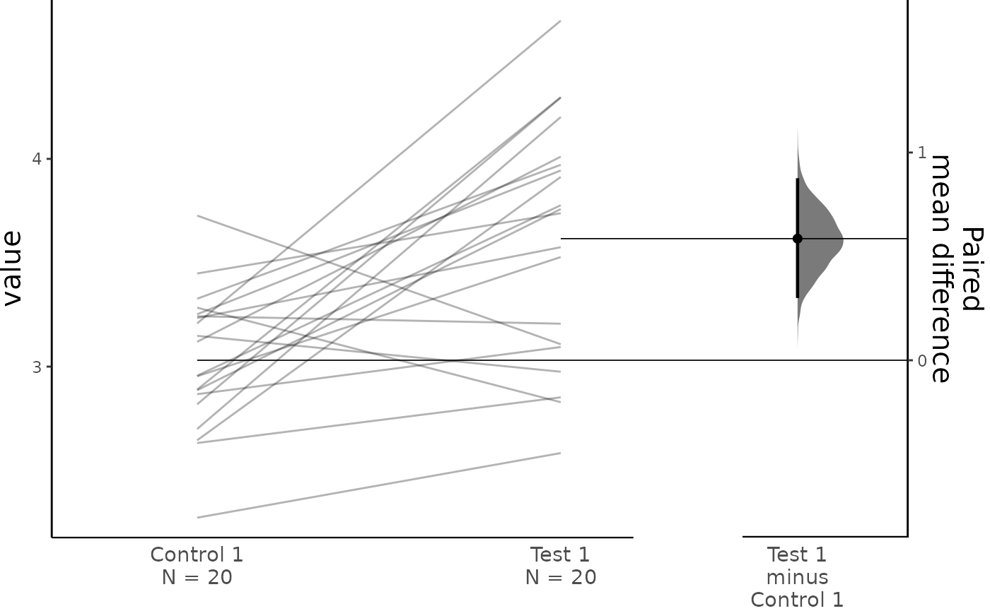
dabest_plot(two_groups_paired_sequential.mean_diff, float_contrast = FALSE,
            raw_marker_size = 0.5, raw_marker_alpha = 0.3,
            contrast_ylim = c(-0.3, 1.3))
dabest_plot(two_groups_paired_baseline.mean_diff,
            raw_marker_size = 0.5, raw_marker_alpha = 0.3)
dabest_plot(two_groups_paired_baseline.mean_diff, float_contrast = FALSE,
            raw_marker_size = 0.5, raw_marker_alpha = 0.3,
            contrast_ylim = c(-0.3, 1.3))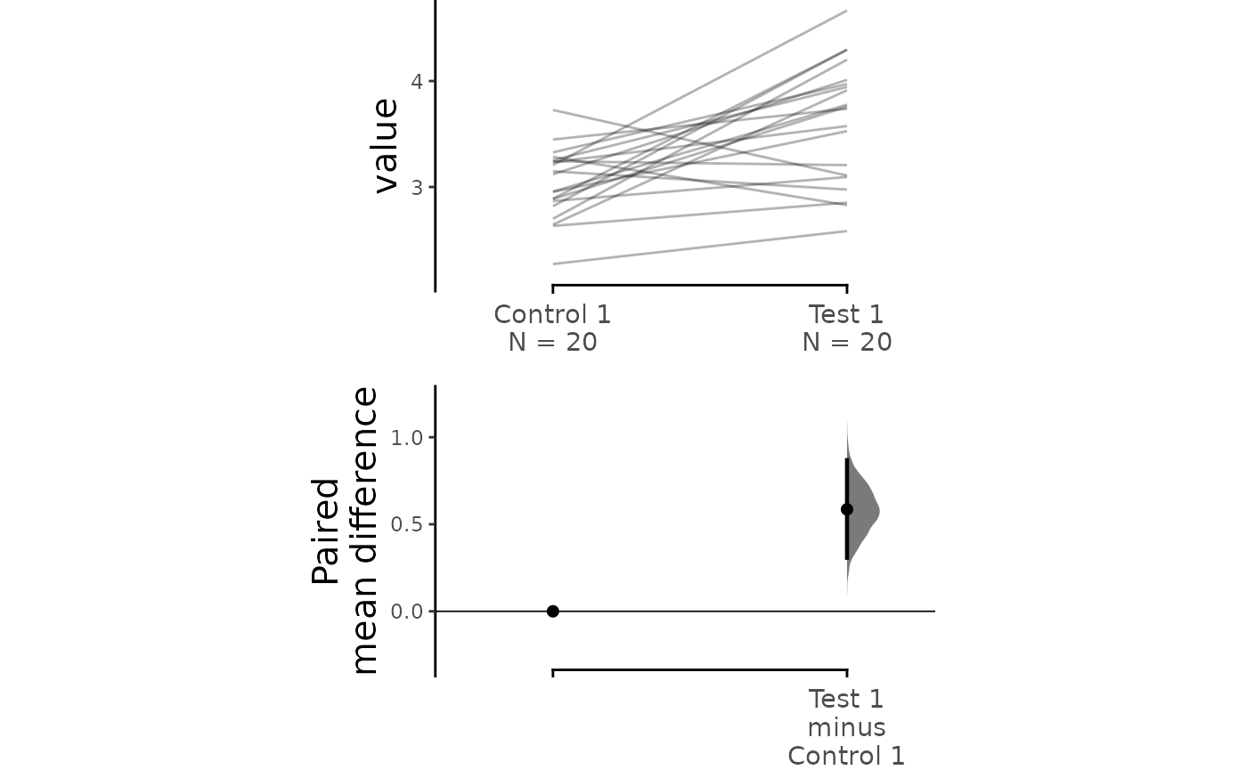
You can also create repeated-measures plots with multiple test
groups. In this case, declaring paired to be “sequential”
or “baseline” will generate the same slopegraph, reflecting the
repeated-measures experimental design, but different contrast plots, to
show the “sequential” or “baseline” comparison:
sequential_repeated_measures.mean_diff <- load(df, x = Group, y = Measurement,
                                     idx = c("Control 1", "Test 1",
                                             "Test 2", "Test 3"),
                                     paired = "sequential", id_col = ID) %>%
  mean_diff()

print(sequential_repeated_measures.mean_diff)
#> DABESTR v0.9.9.9
#> ================
#>
#> Good morning!
#> The current time is 04:27 AM on Tuesday August 22, 2023.
#>
#> The paired mean difference between Test 1 and Control 1 is 0.585 [95%CI 0.307, 0.869].
#> The p-value of the two-sided permutation t-test is c("4e-04", "0.0032", "0.2276"), calculated for legacy purposes only.
#>
#> The paired mean difference between Test 2 and Control 1 is -0.871 [95%CI -1.244, -0.489].
#> The p-value of the two-sided permutation t-test is c("4e-04", "0.0032", "0.2276"), calculated for legacy purposes only.
#>
#> The paired mean difference between Test 3 and Control 1 is 0.293 [95%CI -0.136, 0.713].
#> The p-value of the two-sided permutation t-test is c("4e-04", "0.0032", "0.2276"), calculated for legacy purposes only.
#>
#> 5000 bootstrap samples were taken; the confidence interval is bias-corrected and accelerated.
#> Any p-value reported is the probability of observing the effect size (or greater),
#> assuming the null hypothesis of zero difference is true.
#> For each p-value, 5000 reshuffles of the control and test labels were performed.
#>
#> To get the results of all valid statistical tests, use .mean_diff.statistical_tests
dabest_plot(sequential_repeated_measures.mean_diff,
            raw_marker_size = 0.5, raw_marker_alpha = 0.3)
baseline_repeated_measures.mean_diff <- load(df, x = Group, y = Measurement,
                                             idx = c("Control 1", "Test 1",
                                                     "Test 2", "Test 3"),
                                             paired = "baseline", id_col = ID) %>%
  mean_diff()

print(baseline_repeated_measures.mean_diff)
#> DABESTR v0.9.9.9
#> ================
#>
#> Good morning!
#> The current time is 04:27 AM on Tuesday August 22, 2023.
#>
#> The paired mean difference between Test 1 and Control 1 is 0.585 [95%CI 0.307, 0.869].
#> The p-value of the two-sided permutation t-test is c("4e-04", "0.1312", "0.97"), calculated for legacy purposes only.
#>
#> The paired mean difference between Test 2 and Control 1 is -0.286 [95%CI -0.585, 0.046].
#> The p-value of the two-sided permutation t-test is c("4e-04", "0.1312", "0.97"), calculated for legacy purposes only.
#>
#> The paired mean difference between Test 3 and Control 1 is 0.007 [95%CI -0.323, 0.383].
#> The p-value of the two-sided permutation t-test is c("4e-04", "0.1312", "0.97"), calculated for legacy purposes only.
#>
#> 5000 bootstrap samples were taken; the confidence interval is bias-corrected and accelerated.
#> Any p-value reported is the probability of observing the effect size (or greater),
#> assuming the null hypothesis of zero difference is true.
#> For each p-value, 5000 reshuffles of the control and test labels were performed.
#>
#> To get the results of all valid statistical tests, use .mean_diff.statistical_tests
dabest_plot(baseline_repeated_measures.mean_diff,
            raw_marker_size = 0.5, raw_marker_alpha = 0.3)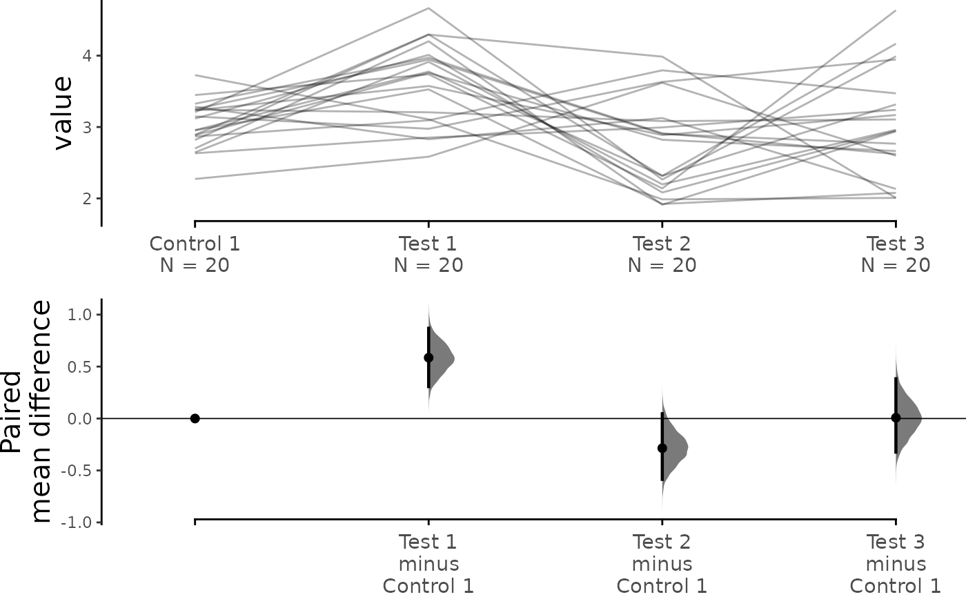
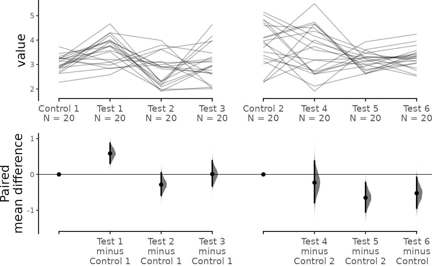
As with unpaired data, dabestr empowers you to perform
complex visualizations and statistics for paired data as well.
multi_baseline_repeated_measures.mean_diff <- load(df, x = Group, y = Measurement,
                                                   idx = list(c("Control 1", "Test 1",
                                                                "Test 2", "Test 3"),
                                                              c("Control 2", "Test 4",
                                                                "Test 5", "Test 6")),
                                                   paired = "baseline", id_col = ID) %>%
  mean_diff()

dabest_plot(multi_baseline_repeated_measures.mean_diff,
            raw_marker_size = 0.5, raw_marker_alpha = 0.3)